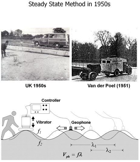
During the very early stage of the surface wave method in 1950s and 60s of using a monotonic vibrator exciting at a single frequency (f) at a time, the
distance (Lf) between two consecutive amplitude maxima was measured by scanning the ground surface with a sensor. Then, corresponding phase
velocity (Cf) was calculated as Cf=Lf * f. This measurement was then repeated for different frequencies to construct a dispersion curve. Underlying
assumption for this approach was the M0-domination of surface waves in the field.
This approach was augmented in the early 1908s by the spectral analysis of surface waves (SASW) method to be more efficient. Instead of trying to
measure the distance of Lf, it tries to measure the phase difference (dp) for a frequency (f) between the two receivers a known distance apart from the
relationship: Cf=2*pi*f/dp (pi=3.14159265). Then, it is repeated for different frequencies to construct a dispersion curve. The same assumption of the
M0-domination of surface waves as used in the earlier times was adopted in the subsequent inversion process during the early stage of the SASW
method. The concept of apparent dispersion curve was, then, introduced in the early 1990s that tried to account for the possibility of multi-modal
influence during the inversion process. The way a dispersion curve is constructed, however, remains basically unchanged.
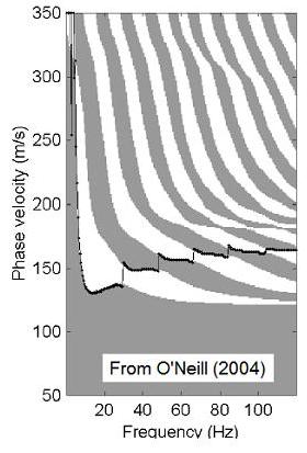
On the other hand, the multichannel approach does not attempt to calculate individual phase velocity first, but constructs an image space where
dispersion trends are identified from the pattern of energy accumulation in this space. Then, necessary dispersion curves are extracted by following
the image trends. All types of seismic waves propagating horizontally are imaged if they take any significant energy noticeable from the relative
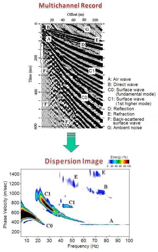
intensity of the image. In this imaging process, a multichannel record in time (t)-space (x) domain is transformed into either frequency (f)-wavenumber
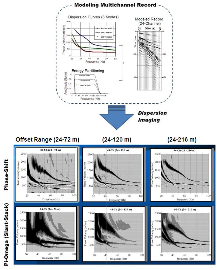
(Kx) or frequency (f)-phase velocity (Cf) domain. The traditional f-k method is the former type, whereas the pi-omega transformation (McMechan and
Yedlin, 1981) and the phase-shift method (Park et al., 1998) are two instances of the latter type. It is generally known that the f-k method results in
the lowest resolution in imaging, whereas the phase-shift method achieves the higher resolution than the pi-omega method (Park et al., 1998; Moro et
al., 2003).
Dispersion Imaging Method (The Phase-Shift Method)
distance (Lf) between two consecutive amplitude maxima was measured by scanning the ground surface with a sensor. Then, corresponding phase
velocity (Cf) was calculated as Cf=Lf * f. This measurement was then repeated for different frequencies to construct a dispersion curve. Underlying
assumption for this approach was the M0-domination of surface waves in the field.
This approach was augmented in the early 1908s by the spectral analysis of surface waves (SASW) method to be more efficient. Instead of trying to
measure the distance of Lf, it tries to measure the phase difference (dp) for a frequency (f) between the two receivers a known distance apart from the
relationship: Cf=2*pi*f/dp (pi=3.14159265). Then, it is repeated for different frequencies to construct a dispersion curve. The same assumption of the
M0-domination of surface waves as used in the earlier times was adopted in the subsequent inversion process during the early stage of the SASW
method. The concept of apparent dispersion curve was, then, introduced in the early 1990s that tried to account for the possibility of multi-modal
influence during the inversion process. The way a dispersion curve is constructed, however, remains basically unchanged.
On the other hand, the multichannel approach does not attempt to calculate individual phase velocity first, but constructs an image space where
dispersion trends are identified from the pattern of energy accumulation in this space. Then, necessary dispersion curves are extracted by following
the image trends. All types of seismic waves propagating horizontally are imaged if they take any significant energy noticeable from the relative
intensity of the image. In this imaging process, a multichannel record in time (t)-space (x) domain is transformed into either frequency (f)-wavenumber
(Kx) or frequency (f)-phase velocity (Cf) domain. The traditional f-k method is the former type, whereas the pi-omega transformation (McMechan and
Yedlin, 1981) and the phase-shift method (Park et al., 1998) are two instances of the latter type. It is generally known that the f-k method results in
the lowest resolution in imaging, whereas the phase-shift method achieves the higher resolution than the pi-omega method (Park et al., 1998; Moro et
al., 2003).
Dispersion Imaging Method (The Phase-Shift Method)
| | | | |
| e-mail: contact@masw.com |
MASW - Dispersion Analysis
This is the first step of data processing in most of surface-wave methods. The goal is to estimate one or more dispersion curves that are in turn
passed into the next step of inversion process, which tries to find a proper layer (shear-velocity, Vs) model whose theoretical dispersion curve(s)
match the measured one(s) as closely as possible. Traditionally, it has been the fundamental-mode (M0) curve usually estimated.
What is dispersion?
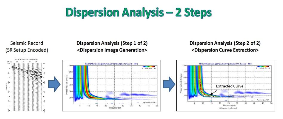
The dispersion analysis itself consists of two steps as illustrated below. The first step generates dispersion image from seismic field record that has
source/recever (SR) setup encoded by using a 2-D (time and space) wavefield transformation method (e.g., phase-shift method, tau-pi transformation,
f-k, etc.). The second step extracts a fundamental-mode (M0) dispersion curve from the image. This extracted curve is called a "measured"
dispersion curve that is an input data to the next data analysis step ("Inversion").
This is the first step of data processing in most of surface-wave methods. The goal is to estimate one or more dispersion curves that are in turn
passed into the next step of inversion process, which tries to find a proper layer (shear-velocity, Vs) model whose theoretical dispersion curve(s)
match the measured one(s) as closely as possible. Traditionally, it has been the fundamental-mode (M0) curve usually estimated.
What is dispersion?
The dispersion analysis itself consists of two steps as illustrated below. The first step generates dispersion image from seismic field record that has
source/recever (SR) setup encoded by using a 2-D (time and space) wavefield transformation method (e.g., phase-shift method, tau-pi transformation,
f-k, etc.). The second step extracts a fundamental-mode (M0) dispersion curve from the image. This extracted curve is called a "measured"
dispersion curve that is an input data to the next data analysis step ("Inversion").
| Dispersion Image Generation by Phase-Shift Method (Park et al., 1998) |