| Fig. 1. |
| Fig. 2. |
The elastic property is usually represented by several independent parameters called elastic moduli—like Young’s, shear, bulk, etc. In practice, however, it is more commonly
represented by more easily measurable physical properties such as seismic P- and S-wave velocities (Vp and Vs) and density (rho), in which Vp and Vs are theoretically
derivable in combination from the elastic moduli and density. It therefore usually refers to these Vp, Vs, and rho when terms like “earth’s property” or “a (layered) earth model”
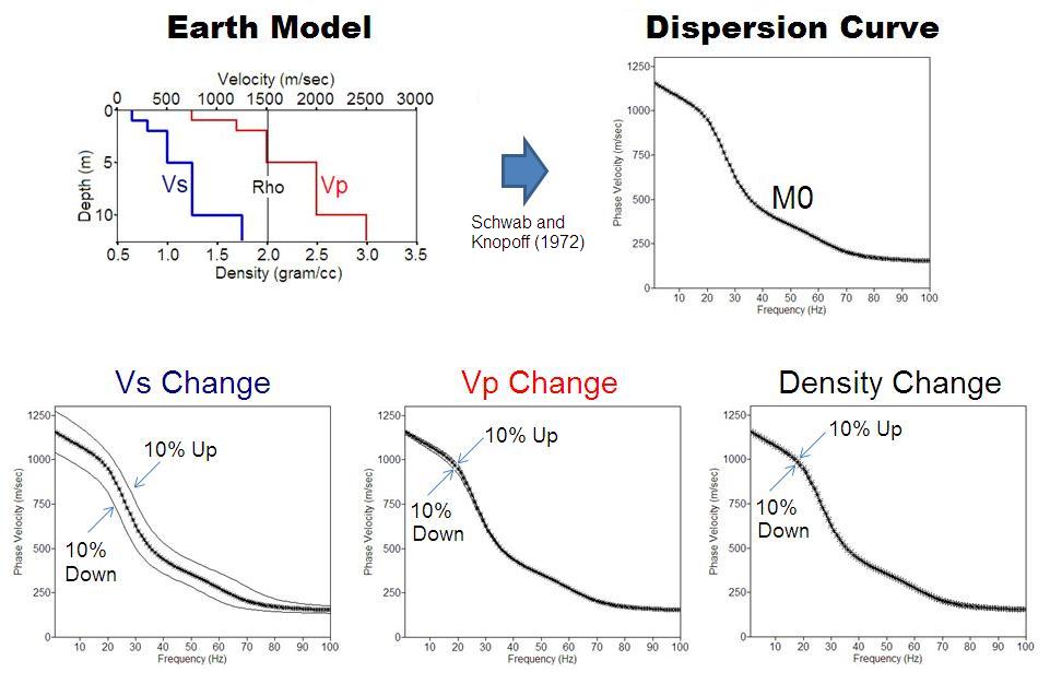
are used in a seismic method. Among these properties, it is usually the S-wave velocity (Vs) that is estimated from the inversion of surface wave data. This is because the type
of data used for the inversion has been the fundamental-mode (M0) dispersion curve, whose shape is determined mostly by the Vs structure of the earth (Fig. 3). A more
accurate expression should be that it has been historically assumed that the fundamental mode dominates in the recorded field data. In consequence, surface wave data
processing has been following this procedure of constructing the M0 curve and then finding the earth’s Vs structure whose theoretical M0 curve most closely matches the
constructed (experimental or measured) M0 curve. S-Velocity (Vs) is one of the critical parameters in geotechnical engineering because it can be a direct indicator of shear and
Young’s moduli, which in turn are often associated with materials’ stiffness and load-bearing capacity of the ground.
represented by more easily measurable physical properties such as seismic P- and S-wave velocities (Vp and Vs) and density (rho), in which Vp and Vs are theoretically
derivable in combination from the elastic moduli and density. It therefore usually refers to these Vp, Vs, and rho when terms like “earth’s property” or “a (layered) earth model”
are used in a seismic method. Among these properties, it is usually the S-wave velocity (Vs) that is estimated from the inversion of surface wave data. This is because the type
of data used for the inversion has been the fundamental-mode (M0) dispersion curve, whose shape is determined mostly by the Vs structure of the earth (Fig. 3). A more
accurate expression should be that it has been historically assumed that the fundamental mode dominates in the recorded field data. In consequence, surface wave data
processing has been following this procedure of constructing the M0 curve and then finding the earth’s Vs structure whose theoretical M0 curve most closely matches the
constructed (experimental or measured) M0 curve. S-Velocity (Vs) is one of the critical parameters in geotechnical engineering because it can be a direct indicator of shear and
Young’s moduli, which in turn are often associated with materials’ stiffness and load-bearing capacity of the ground.
| Fig. 3. |
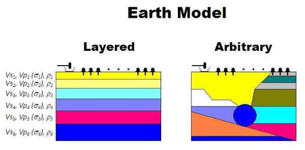
It is the 1D (depth) variation that is found for the Vs structure
because the measured curve is most sensitive to the vertical
variation of Vs and lateral variation is largely averaged off during
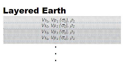
data processing. This type of 1D Vs model is often referred as a
layered earth model, which may include Vs, Vp, and rho all
together or simply Vs alone with others fixed. A layered earth
model inevitably carries no lateral variation as the case with an
arbitrary earth model (Fig. 4). This means the surface wave
method gives the 1D Vs structure (also called profile) most
representative of the subsurface materials below the receiver
spread by approximating them as a layered earth model despite
the fact that, in reality, a certain degree of lateral variation always
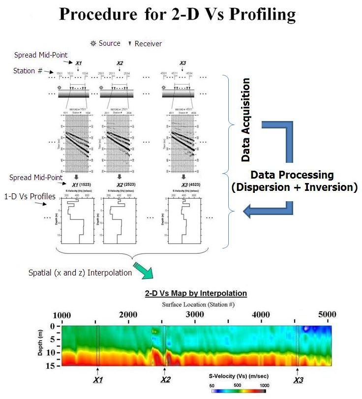
exists. Because of the nature of multichannel processing, it is
usually the center location of the receiver spread to which this 1D
Vs profile is assigned as the most representative surface
location if the coordinate information is necessary. With
accumulation of multiple number of this 1D Vs profile assigned
with a unique surface coordinate, a 2D Vs profile is constructed
by using an appropriate spatial interpolation scheme.
because the measured curve is most sensitive to the vertical
variation of Vs and lateral variation is largely averaged off during
data processing. This type of 1D Vs model is often referred as a
layered earth model, which may include Vs, Vp, and rho all
together or simply Vs alone with others fixed. A layered earth
model inevitably carries no lateral variation as the case with an
arbitrary earth model (Fig. 4). This means the surface wave
method gives the 1D Vs structure (also called profile) most
representative of the subsurface materials below the receiver
spread by approximating them as a layered earth model despite
the fact that, in reality, a certain degree of lateral variation always
exists. Because of the nature of multichannel processing, it is
usually the center location of the receiver spread to which this 1D
Vs profile is assigned as the most representative surface
location if the coordinate information is necessary. With
accumulation of multiple number of this 1D Vs profile assigned
with a unique surface coordinate, a 2D Vs profile is constructed
by using an appropriate spatial interpolation scheme.
| Fig. 4. |
This type of M0-curve based inversion used to find the 1D Vs profile has been the most typical approach historically adopted, and this is currently the case with the MASW
method as well. This, however, does not necessarily mean it is the only viable approach with the MASW method. In fact, there are several other approaches currently being
researched or already under routine use that use other types of surface wave data rather than the M0 curve either separately or in combination. They include
Multimodal Inversion
Dispersion Image Inversion
Raw Data Inversion
2D Vs Inversion
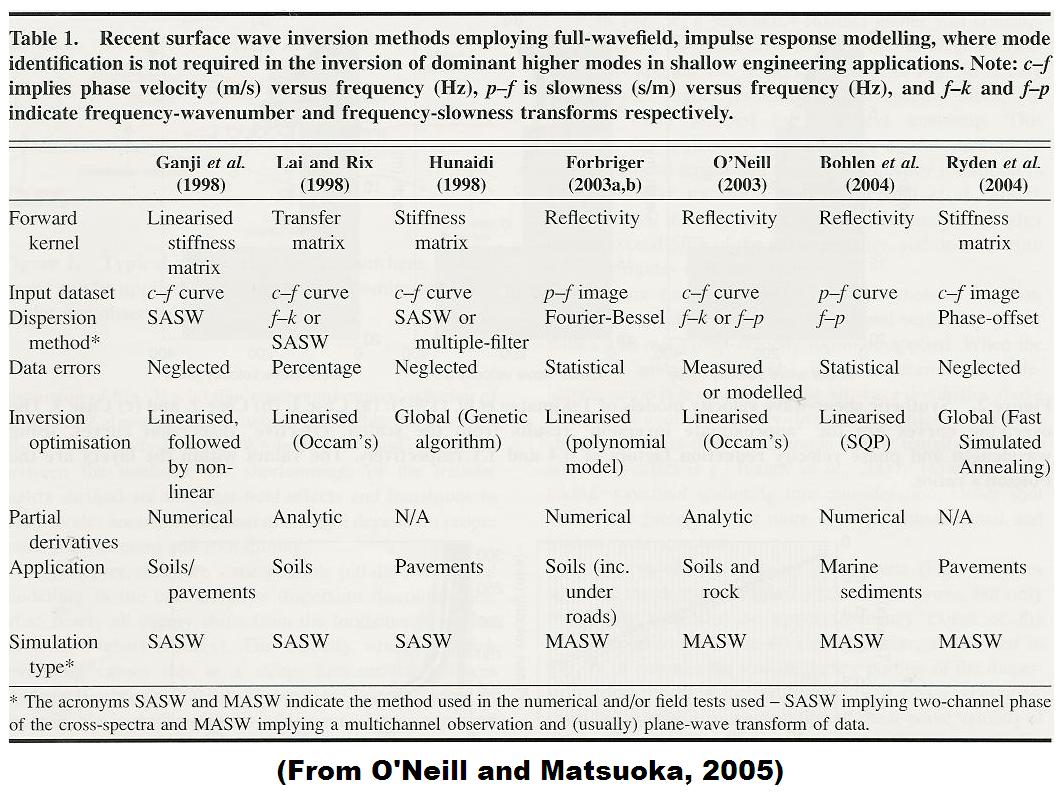
The special edition in 2005 on the surface wave method published by the Journal of Environmental and Engineering Geophysics (JEEG) presents a summary table of typical
inversion approaches adopted in both the two-receiver (SASW) and the multichannel (MASW) methods. Regardless of any specific type used, the surface wave inversion is
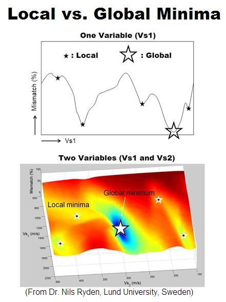
non-unique and non-linear problem to varying extent under different circumstances. In addition, it is not guaranteed if a final solution indeed represents the global minimum
instead of one of the local minima.
method as well. This, however, does not necessarily mean it is the only viable approach with the MASW method. In fact, there are several other approaches currently being
researched or already under routine use that use other types of surface wave data rather than the M0 curve either separately or in combination. They include
Multimodal Inversion
Dispersion Image Inversion
Raw Data Inversion
2D Vs Inversion
The special edition in 2005 on the surface wave method published by the Journal of Environmental and Engineering Geophysics (JEEG) presents a summary table of typical
inversion approaches adopted in both the two-receiver (SASW) and the multichannel (MASW) methods. Regardless of any specific type used, the surface wave inversion is
non-unique and non-linear problem to varying extent under different circumstances. In addition, it is not guaranteed if a final solution indeed represents the global minimum
instead of one of the local minima.
MASW - Inversion Analysis
What is inversion in general?
Typical MASW Inversion Multi-modal Inversion Dispersion Image Inversion Raw Data Inversion 2D-Vs Inversion
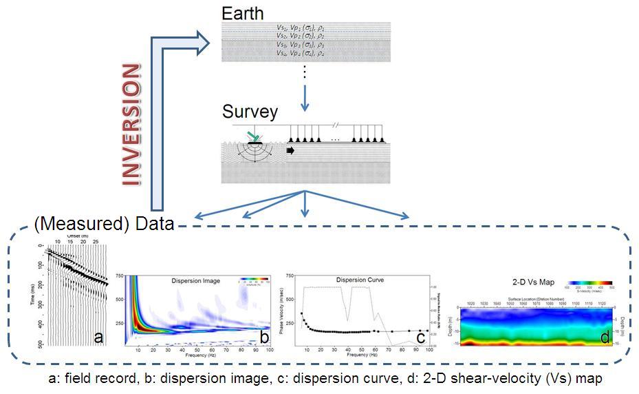
Historically, the inversion of surface waves has meant an estimation of the earth’s properties from the measured surface wave data (Fig. 1). It is the earth’s elastic property that
is estimated among many properties—electric and magnetic to name a few. Various types of surface wave data can be used for the estimation that may include raw field
record, dispersion image, dispersion curve(s), and a preliminary 2D shear(S)-wave velocity (Vs) map (see different inversion approaches listed below). Regardless of the type
of data used, the surface wave inversion cannot be solved directly, requiring an optimization technique to find the most probable solution in a pool of infinite candidates. This
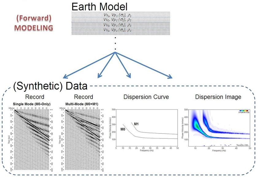
technique can be a deterministic approach, random, or combination of both. On the other hand, the forward modeling (Fig. 2) of surface wave phenomena is usually a unique
problem.
What is inversion in general?
Typical MASW Inversion Multi-modal Inversion Dispersion Image Inversion Raw Data Inversion 2D-Vs Inversion
Historically, the inversion of surface waves has meant an estimation of the earth’s properties from the measured surface wave data (Fig. 1). It is the earth’s elastic property that
is estimated among many properties—electric and magnetic to name a few. Various types of surface wave data can be used for the estimation that may include raw field
record, dispersion image, dispersion curve(s), and a preliminary 2D shear(S)-wave velocity (Vs) map (see different inversion approaches listed below). Regardless of the type
of data used, the surface wave inversion cannot be solved directly, requiring an optimization technique to find the most probable solution in a pool of infinite candidates. This
technique can be a deterministic approach, random, or combination of both. On the other hand, the forward modeling (Fig. 2) of surface wave phenomena is usually a unique
problem.
| | | | | | | |